2019-数据结构-数据结构8.0-graphs
Graphs
1. 图的定义
- Graph = (V, E)
- V: nonempty finite vertice set(顶点集) 一个非空确定顶点个数的集合
- E: edge set(边集)
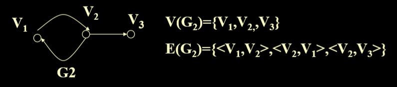
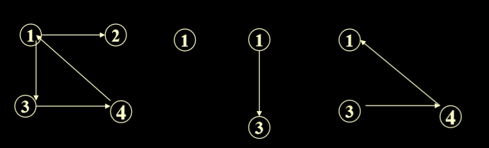
1.1. 有向图
- If the tuple denoting an edge is ordered, then <v1,v2> and <v2,v1> are different edges. (如果表示的边的元组是有序的,也就是<v1,v2>和<v2,v1>是不同的)
- v1: 有向图边的始点
- v2: 有向图边的终点
- In a directed graph with n nodes, the number of edges <=n*(n-1). If “=” is satisfied, then it is called a complete directed graph.(一个有n个节点的有向图,其边的个数<= n*(n-1),如果相等,则为是一个完全有向图)
- 完全图(有向完全图):指有向图中每两个顶点都相互指向。
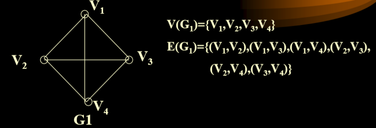
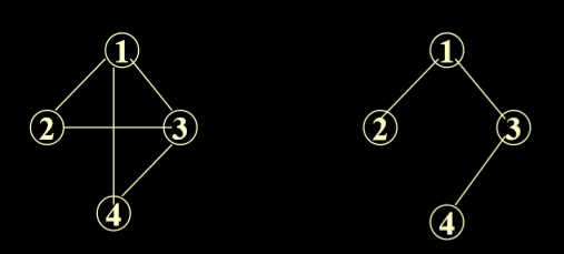
1.2. 无向图
- If the tuple denoting an edge is unordered, then (v1,v2) and (v2,v1) are the same edge.(如果表示边的元组是无序的,则(v1,v2)和(v2,v1)是相同的边。)
- In an undirected graph with n nodes, the number of edges <= n*(n-1)/2. If “=” is satisfied, then it is called a complete undirect graph.(在一个有n个顶点的无向图中,边的个数 <= n(n-1)/2,如果刚好相等,则被称为完全无向图)
- 完全图(无向完全图):就是指每两个顶点之间都有一条边。
1.3. 其他图
- 以下两种图在我们的数据结构中不进行讨论
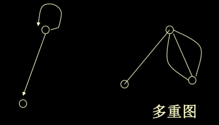
- 不考虑 自环(ring) 和 多重边 的多重图。
1.4. 顶点的度数
- 对于无向图只有度数,而对于有向图不仅仅有入度,还有出度。
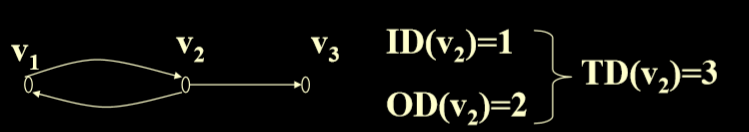
- degree dv of vertex v, TD(v): is the number of edges incident on vertex v. In a directed graph :(顶点v的度数为dv,TD(V)是顶点v的度数,在有向图中)
- in-degree of vertex v is the number of edges incident to v, ID(v).(顶点v的入度是指向顶点v的边的个数)
- out-degree of vertex v is the number of edges incident from the v, OD(v). (顶点v的出度从v出发的边的个数)
- 性质:(度数)TD(v)=ID(v)+OD(v)
1.5. 图的性质
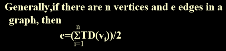
- 所有的度数加起来是边的个数的两倍。
1.6. 子图
- Graph G=(V,E),G’=(V‘,E‘), if V’包含于V, E’包含于E, and the vertices incident on the edges in E’ are in V’, then G’ is the subgraph of G. For example: 如果图G和图G’,如果V’包含于V,E’包含于E,并且E’中顶点的边也在G’中,那么G’是G的子图
1.7. 路径(path)
- A sequence of vertices P=i1,i2,……ik is an i1 to ik path in the graph of graph G=(V,E) iff the edge(ij,ij+1)is in E for every j, 1 <= j < k.(在图 G=(V,E)中,如果每j的边(ij,ij+1)在E中,1<= j< k,则顶点序列P=i1,i2,…,ik是i1到ik的路径。)
1.8. 简单路径和环(Simple path and cycle)
- A Simple path is a path in which all vertices except possibly the first and last , are different.(简单路径 : 路径除了第一个和最后一个顶点中没有出现相同的顶点)
- A Simple cycle is a simple path with the same start and end vertex.(简单回路:起点和终点相同的时候的简单路径)
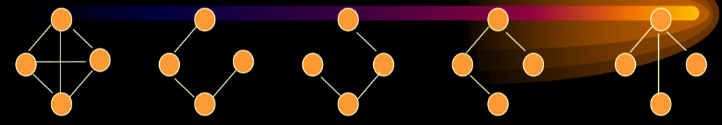
1.9. 连通图和连通分量(Connected graph & Connected component)
- In a undirected graph, if there is a path from vertex v1 to v2, then v1 and v2 are connected.(在无向图中,如果v1到v2之间有一条路径,那么v1和v2是连通的)
- In a undirected graph ,if two arbitrary vertices are connected, then the graph is a connected graph(在无向图中,如果任意两个顶点是连通的,则该图是连通图)
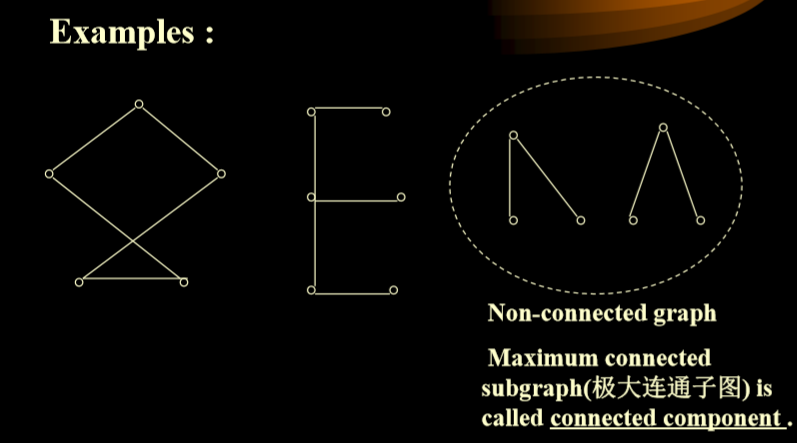
- 极大连通子图:就是结点个数最多的连通的子图。
1.10. 强联通图和强联通分量(Strong connected graph and strongly connected component)
- A digraph is strongly connected iff it contains a directed path from i to j and from j to i for every pair of distinct vertices i and j.(有向图是强连通的,当它包含从 i 到 j 和从 j 到 i 的有向路径时,对于每对不同的顶点 i 和 j)。
- 简单来说就是既要过的去,也要回得来
- The maximum strong connected subgraph (极大强连通子图) of a non-strongly connected graph is called strongly connected conponent (强连通分量).(一个非强连通图的最大强连通子图(South-South-PosialSuth-Posiple Fug)称为强连通构(Suth-Posiple Stand))
1.11. 加权图(Network)
- When weights and costs are assigned to edges, the resulting data object is called weighted graph and weighted digraph.(当权值和代价分配给边时,得到的数据对象称为加权图和加权有向图。)
- The term network refers to weighted connected graph and weighted connected digraph. (网络是用来代指加权连通图和加权连通有向图)

1.12. 生成树(Spanning tree)
- A spanning tree of a connected graph is its minimum connected subgraph(最小连通子图). An n-vertex spanning tree has n-1 edges. (连通图的生成树是其最小连通子图。n顶点生成树有n-1条边。)
- 保持联通的最小边数的图
2. ADT Graph and Digraph 无向图和无向图的抽象逻辑
1 | |
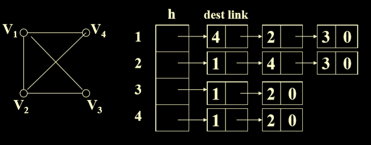
3. 图的表示与实现(Representation of graphs and digraphs)
- 有向图(graphs)
- 无向图(digraphs)
3.1. 邻接矩阵(Adjacency Matrix)
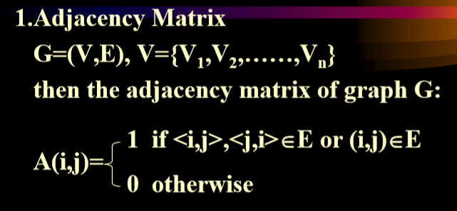
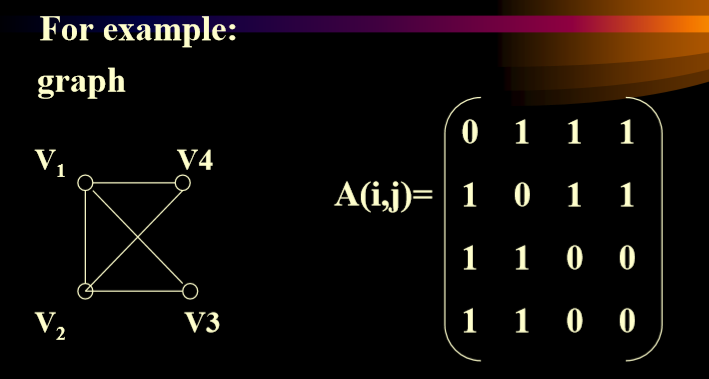
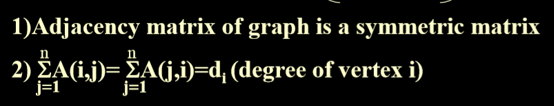
- 无向图的邻接矩阵
- 无向图的每个顶点的度数等于矩阵中每一行的和。
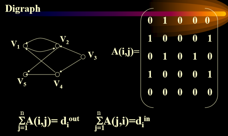
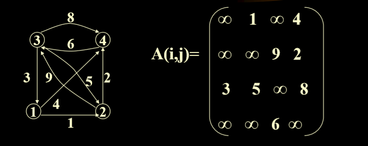
- 有向图的邻接矩阵
- 出度对行求和
- 入度对列求和
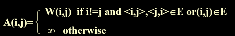
- 加权图(网络)的邻接矩阵
- 注意使用的无穷标识没有通路
- 当节点数很大,边很少的时候不适用于邻接矩阵。
3.1.1. 邻接矩阵性质
- 无向图的邻接矩阵是对称的。
3.2. 其他需要的结构
- 一个记录各顶点信息的表
- 一个当前的边数
3.3. 邻接矩阵实现的代码
1 | |
3.3.1. 需要实现的方法
- 构造方法
1 | |
- 求顶点V的第一个邻接顶点的位置
1 | |
3.4. 邻接表实现
- reduce the storage requirement if the number of edges in the graph is small.当无向图中的边的个数比较少的时候,降低存储需要的空间的量
- Eg.无向图的例子
- cost是指权重
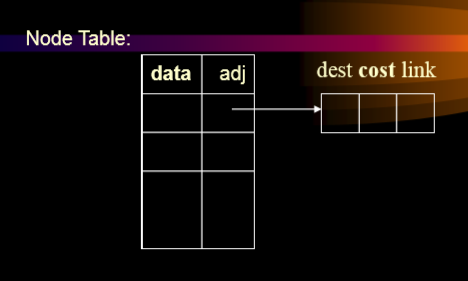
3.4.1. 邻接表的声明
1 | |
3.4.2. 图的类定义
1 | |
3.4.3. 部分实现的方法
- 构造方法
1 | |
- 根据数据值找到下标
1 | |
- 给出顶点V的第一个邻接顶点的位置
1 | |
- 找到下一个邻居
1 | |
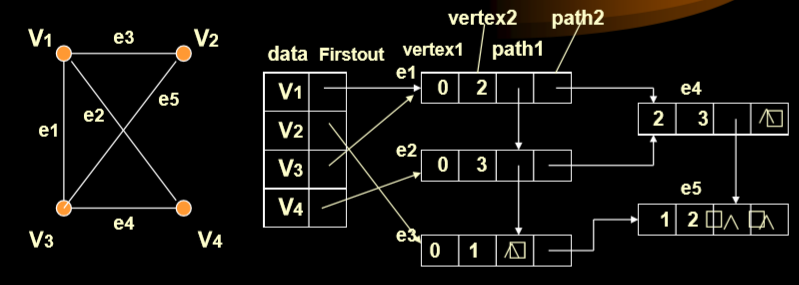
3.5. 邻接多重表
- 在无向图中, 如果边数为m, 则在邻接表表示中需2m个单位来存储. 为了克服这一缺点, 采用邻接多重表, 每条边用一个结点表示.
- 其中的两个结点号就是边的两个点。
- path1指向的就是同样始点(vertex1),顺序终点的结果。
- path2执行的是以vertex2为始点顺序向下的。
- Eg.使用正常的邻接表,则右边应该有10个点,但是多种表就是只有5个表
- 默认情况下边的始点的编号要小于终点的编号大小。
- 对有向图而言,需用邻接表和逆邻接表,如果把这两个表结合起来用有向图的邻接多重表(也称为十字链表)来表示一个有向图.
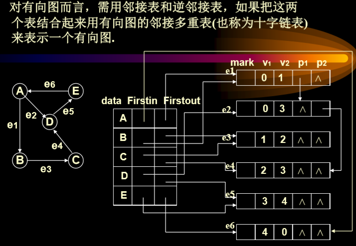
- 邻接表和邻接多重表之间的区别在于有几个顶点,有几个边。
- data部分只记录first-in和first-out,也就是第一条出边和第一条入边。
4. 图的遍历和连通性
- 图的遍历 (Graph Traversal): 从图中某一顶点出发访问图中其余顶点,且使每个顶点仅被访问一次.

- 树的遍历,左子女右兄弟。
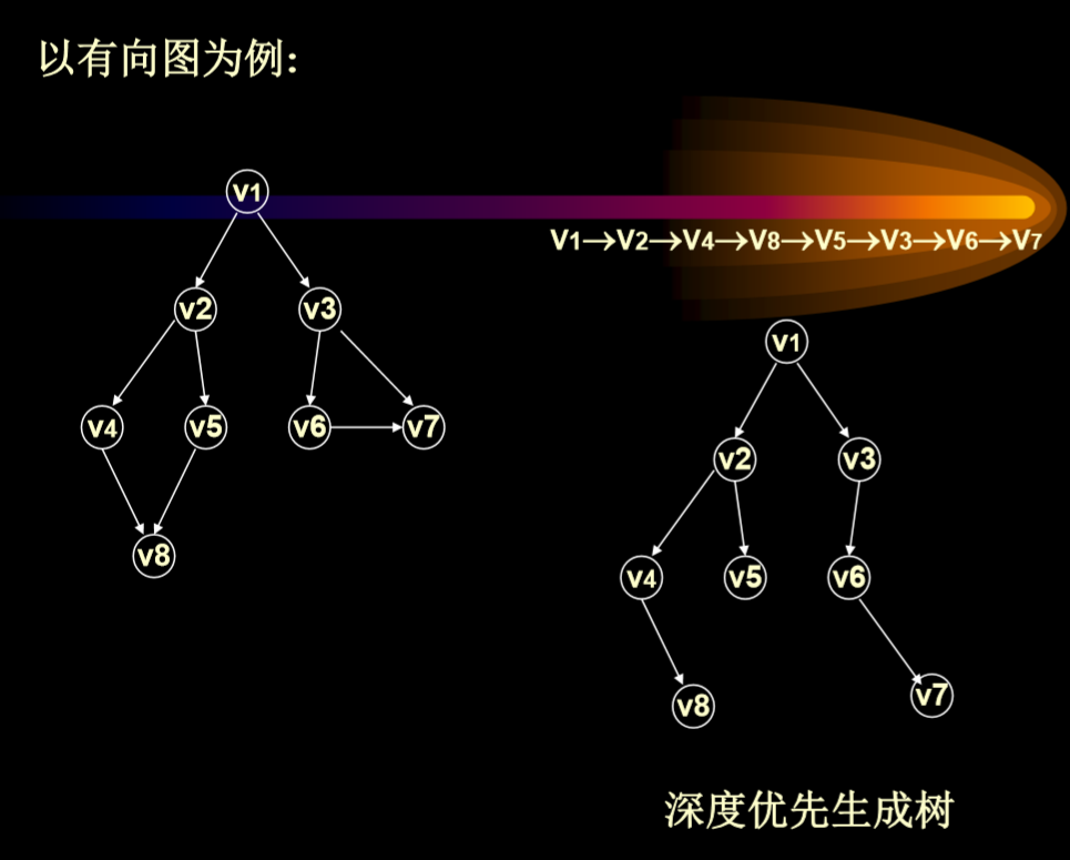
4.1. DFS(depth-first-search,深度优先搜索)
4.1.1. 算法思想
- 从图中某个顶点V0出发,访问它,然后选择一个
V0邻接到的未被访问的一个邻接点V1出发深度优先遍
历图,当遇到一个所有邻接于它的结点都被访问过了的
结点U时,回退到前一次刚被访问过的拥有未被访问的
邻接点W,再从W出发深度遍历,……直到连通图中的所
有顶点都被访问过为止.
- 递归方法实现 算法中用一个辅助数组visited[]:
- 0:未访问
- 1:访问过了
- 我们假设图为连通图
4.1.2. 算法实现
1 | |
4.1.3. 算法分析
- 用邻接表表示 O(n+e)
- 用邻接矩阵表示 O(n2)
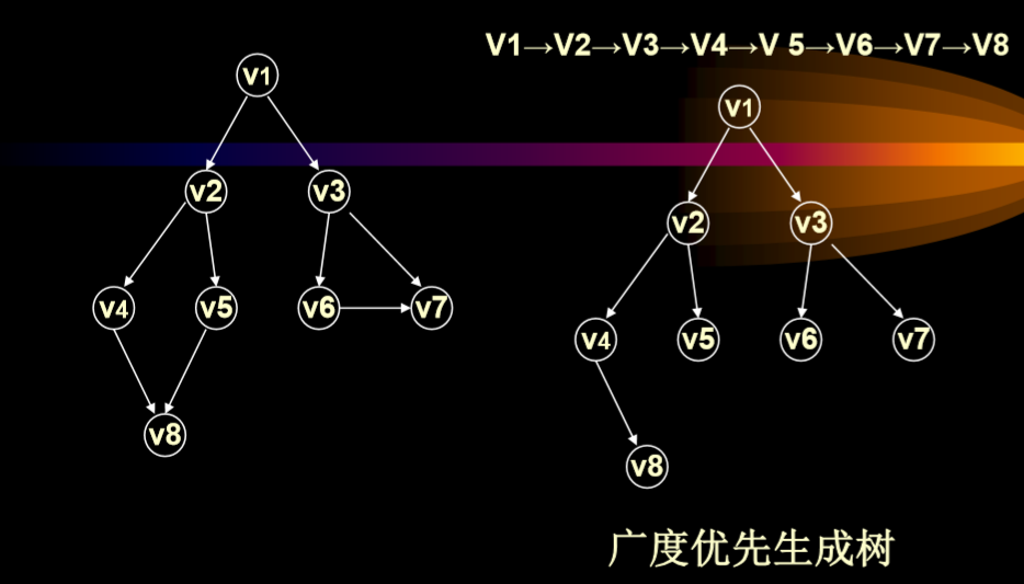
4.2. 广度优先搜索(Breadth search)
4.2.1. 思想
- 从图中某顶点V0出发,在访问了V0之后依次访
问v0的各个未曾访问过的邻接点,然后分别从这些邻接
点出发广度优先遍历图,直至图中所有顶点都被访问
到为止.
- 算法同样需要一个辅助数组visited[] 表示顶点是否被访问过. 还需要一个队列,记正在访问的这一层和上一层的顶点. 算法显然是非递归的.
1 | |
4.2.2. 算法分析
- 每个顶点进队列一次且只进一次,∴算法中循环语句至多执行n次。
- 从具体图的存储结构来看
- 如果用邻接表:O(n+e)
- 如果用邻接矩阵: 对每个被访问过的顶点,循环检测矩阵中n个元素,∴时间代价为 O(n2)
4.3. 连通分量
- 以上讨论的是对一个无向的连通图或一个强连通图的有向图进行遍历,得到一棵深度优先或广度优先生成树.
但当无向图(以无向图为例)为非连通图时,从图的某一
顶点出发进行遍历(深度,广度)只能访问到该顶点所在
的最大连通子图(即连通分量)的所有顶点. - 下面是利用深度优先搜索求非连通图的连通分量算法 实际上只要加一个循环语句就行了.
1 | |
5. 最小生成树
5.1. 生成树
5.1.1. 生成树的定义
- 设G =(V,E)是一个连通的无向图(或是强连通有向图) 从图G中的任一顶点出发作遍历图的操作,把遍历走过的边的集合记为TE(G),显然 G‘=(V,TE)是G之子图, G‘被称为G的生成树(spanning tree),也称为一个连通图.
- n个结点的生成树有n-1条边。
- 生成树的代价(cost):TE(G)上诸边的代价之和
- 生成树不唯一
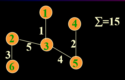
5.1.2. 最小代价生成树
- 各边权的总和为最小的生成树
5.2. 贪心(Grandy)求解最小代价生成树
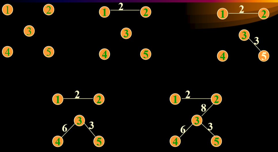
- 6个城市已固定,现从一个城市发出信息到每一个城市如何选择或铺设通信线路,使花费(造价)最低。
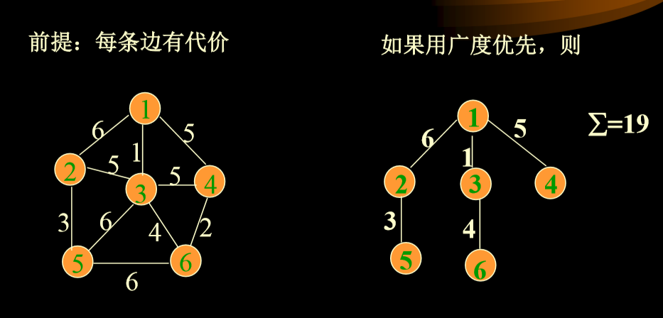
- 两个算法:Prim, Kruskal.
- 算法思想:贪心算法(逐步求解)
5.2.1. 贪心策略的具体内容
- Grandy策略:设:连通网络N={V,E}, V中有n个顶点。
- 先构造 n 个顶点,0 条边的森林 F ={T0,T1,……,Tn-1}
- 每次向 F 中加入一条边。该边是一端在 F 的某棵树Ti上而另一端不在Ti上的所有边中具有最小权值的边。 这样使F中两棵树合并为一棵,树的棵数 - 1
- 重复上述操作n-1次
- 去掉所有边,每次加入的边是当前最小的边,并且保证这个边不是回边。
5.2.2. 最小生成树的类声明
1 | |
- 边结构:tail + head + cost
1 | |
5.3. Kruskal算法(对边进行排序,然后生成)
- 把无向图的所有边排序
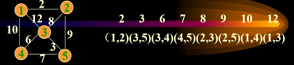
- 一开始的最小生成树为

- 在E中选一条代价最小的边(u,v)加入T,一定要满足(u,v) 不和TE中已有的边构成回路
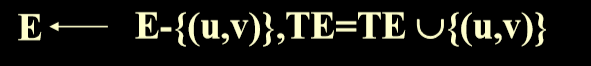
- 一直到TE中加满n-1条边为止。
5.3.1. 代码实现
1 | |
1 | |
5.3.2. 算法分析
- 建立e条边的最小堆
- 检测邻接矩阵O(n2)
- 每插入一条边,执行一次 fiterup() 算法:log2e 所以,总的建堆时间为O(elog2e)
- 构造最小生成树时
- e次出堆操作:每一次出堆,执行一次filterdown(), 总时间为O(elog2e)
- 没有考虑悬挂问题
- 2e次find操作:O(elog2n),树高是log2n
- 从头开始生成,两个高为1的树,做union,才有高度为2的树
- 两个高为2的树,做union,才有高度为3的树
- 树的高度最坏情况下是log2n,当切仅当第一个二叉树
- n-1次union操作:O(n)
- 所以,总的计算时间为O(elog2e+elog2n+n2+n)
- e次出堆操作:每一次出堆,执行一次filterdown(), 总时间为O(elog2e)
5.4. 物理实现
- 图用邻接矩阵表示,edge(边的信息)
- 图的顶点信息在顶点表 Verticelist中
- 边的条数为CurrentEdges
- 取最小的边以及判别是否构成回路,
- 取最小的边利用:最小堆(MinHeap)
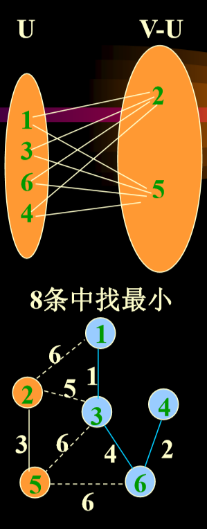
5.5. Prim算法(结合顶点,考虑所有可达的边的权重大小)
- 设:原图的顶点集合V(有n个)生成树的顶点集合U(最后也有n个),一开始为空TE集合为{}
- 步骤:
- U={1}任何起始顶点,TE={}
- 每次生成(选择)一条边。这条边是所有边(u,v) 中代价(权)最小的边, u∈U,v∈V-U TE=TE+[(u,v)]; U=U+[v]
- 当U≠V,返回上面一个步骤
5.5.1. 例子
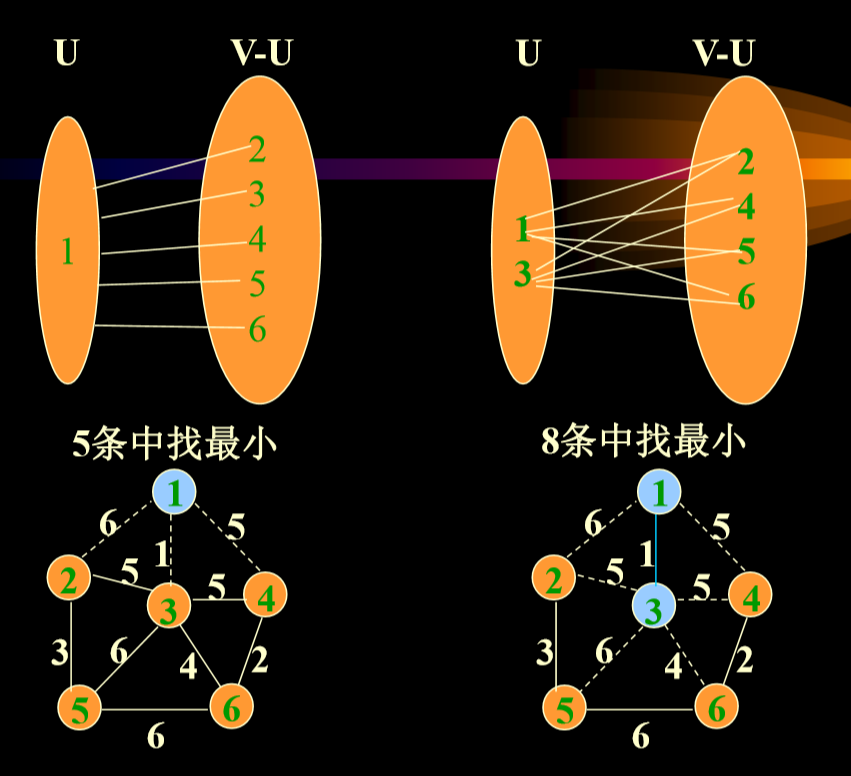
- 一开始只考虑从1号顶点到其他顶点之间的边。
- 泛泛而言,考虑u和v之间的边
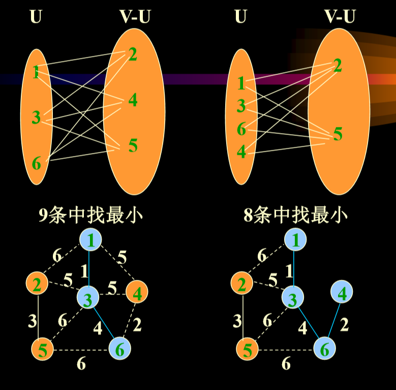
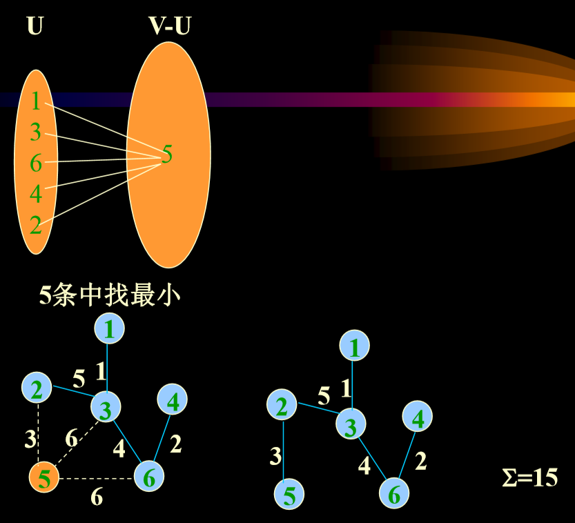
5.5.2. 最小生成树不唯一
- 对于一般的图来讲,最小生成树不唯一。
- 所以相应的Prime算法和Kruskal算法也会出现多解得 情况。
5.5.3. 算法分析
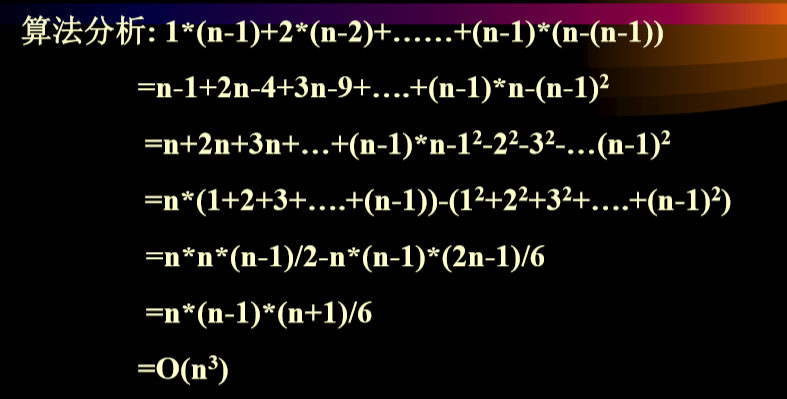
- 第一次的时候u只有1个元素,而第二次则有2个,以此类推。
- 使用邻接矩阵实现的图,可以把时间复杂度降低到O(n2)
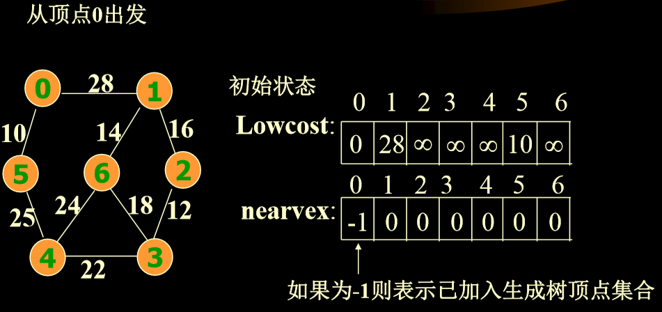
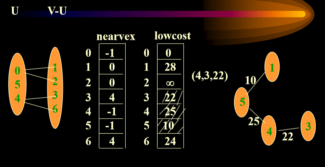
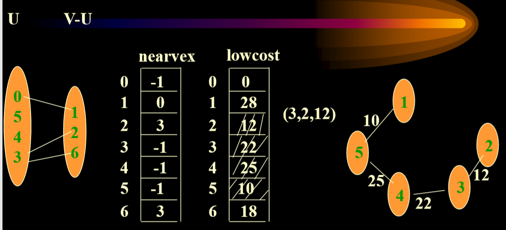
5.6. Prim算法优化
- 使用两个数组Lowcost[ ]、nearvex[ ]
- Lowcost[]:存放生成树顶点集合内顶点到生成树外各顶点的边上的当前最小权值
- nearvex[]:记录生成树顶点集合外各顶点,距离集合内那个顶点最近。
-
拿u为1364为例,将2拉入u之后,如果1364到5的最小值小于2到5之间的距离,则抛弃25边,否则更新数组。
-
对于nearvex:记录的结点,lowcost对应记录的是相应边的权重(按照上面的序号)
- 更新最小边:发生在加入新的结点的时候,需要在nearvex中更新对应位置的最小边。
5.6.1. 算法实现
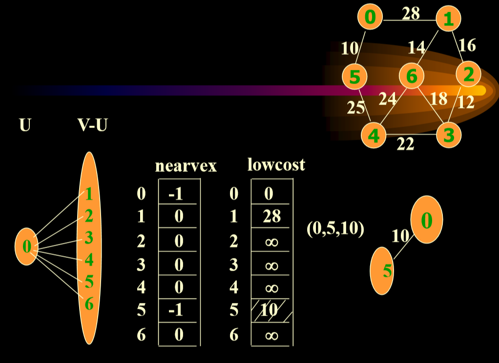
- 在Lowcost[ ]中选择nearvex[i]不等于-1,且lowcost[i] 最小的边用v标记它。,则选中的权值最小的边为(nearvex[v],v), 相应的权值为lowcost[v]。 例如在上面图中第一次选中的v=5;则边(0,5),是选中的权值最小的边,相应的权值为lowcost[5]=10。 反复做以下工作
- 将nearvex[v] 改为-1,表示它已加入生成树顶点集合。将边(nearvex[v],v,lowcost[v])加入生成树的边集合。
- 修改。取lowcost[i]=min{lowcost[i],Edge[v][i]},即用生成树顶点集合外各顶 点i到刚加入该集合的新顶点 v的距离(Edge[v][i])与原来它所到生成树顶点 集合中顶点的最短距离lowcost[i]做比较,取距离近的,作为这些集合外顶 点到生成树顶点集合内顶点的最短距离。
- 如果生成树顶点集合外的顶点i到刚加入该集合新顶点v的距离比原来它 到生成树顶点集合中顶点的最短距离还要近,则修改nearvex[i]: nearvex[i]=v 表示生成树外顶点i到生成树的内顶点v 当前距离最短。
5.6.2. 示例
- 4->5 25<正无穷,更新
- nearvex更新顶点,lowcost更新权值
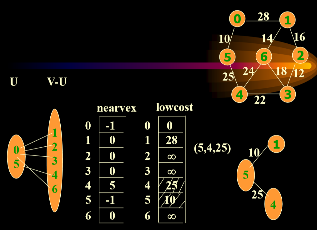
- 考虑1->4、2->4等等


5.6.3. Prim算法实现
1 | |
5.6.4. 估计算法复杂度
- 第一个for循环的复杂度是O(n)的
- 第二个嵌套的for循环的复杂度是O(n2)的
6. 最短路径
- 设G=(V,E)是一个带权图(有向,无向),如果从顶点v到顶点w的一条路径为(v,v1,v2,…,w),其路径长度不大于从v到w的所有其它路径的长度,则该路径为从 v 到 w 的最短路径。
- 背景:在交通网络中,求各城镇间的最短路径。
- 三种算法:
- 边上权值为非负情况的从一个结点到其它各结点的最短路径 (单源最短路径)(Dijkstra算法)
- 边上权值为任意值的单源最短路径
- 边上权值为非负情况的所有顶点之间的最短路径
6.1. 含非负权值的单源最短路径(Dijkstra)
- 问题
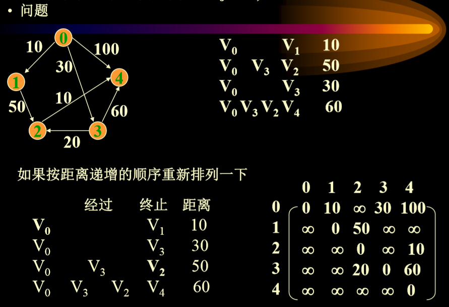
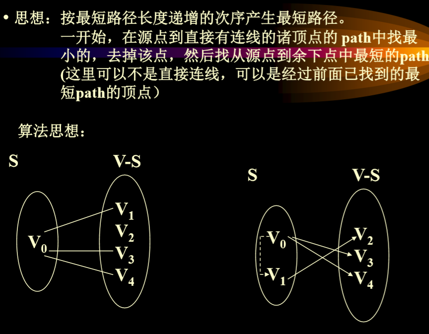
6.1.1. 贪心思想
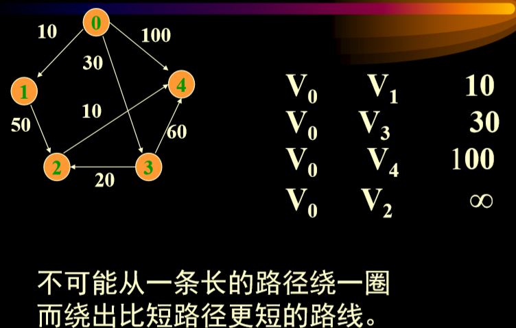
- 起点V0,首先直接连接,不管是否直接连接。
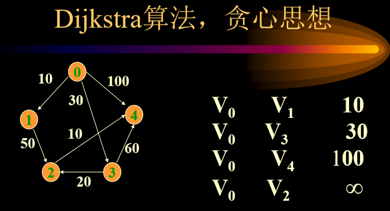
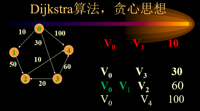
- 排好序后,V0-V1 10已经是最小的了,不可能再找到更短的路径
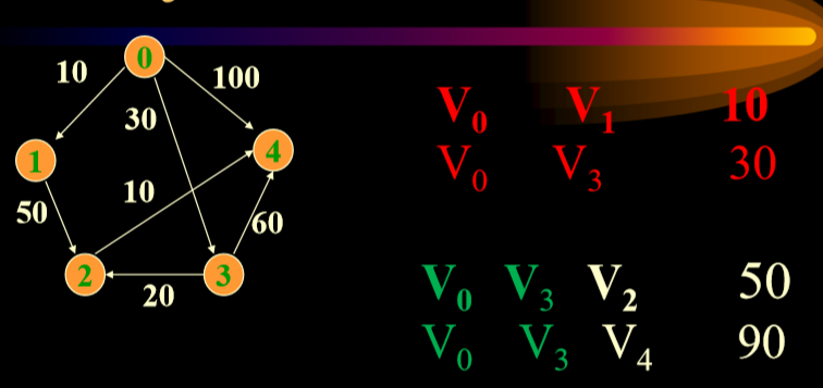
- 接下来,尝试V0-v2通过V1绕会不会比原来的更短(考虑V1-V2直连),V0-V4从V1绕会不会比原来更短(考虑V2-V3直连),如果短则更新,此时V0-V3是三者中最小值,所以选择V0-V3。
- 尝试绕行V3,计算直连,更新掉,然后重复
- 红色是已经选择好的,绿色是绕行选择。
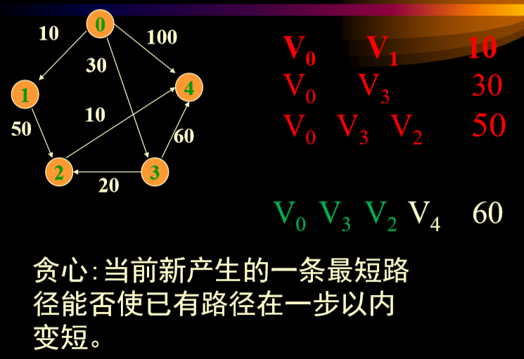
- 进一步思考,就是只进行一步,不进行多不步。
- 总体来讲:不可能走更长的路径,然后回来

- 数值更新,路径数组对应位置更新
6.1.2. 代码实现
1 | |
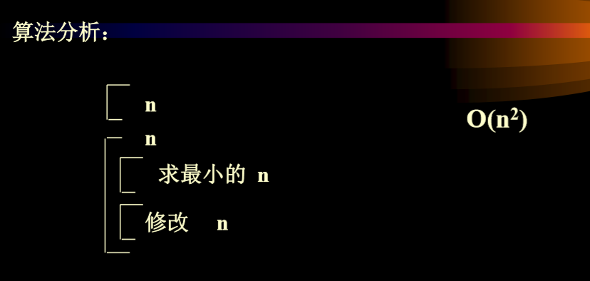
6.1.3. 算法复杂度分析
6.2. 贝尔曼——福特改进算法
- 边上权值为任意值的单源最短路径(贝尔曼—福特) dijkstra算法在边上权值为任意值的图上是不能正常工作的。
- dist1[u],dist2[u],…distn-1[u]
- dist1[u]:是从源点v到终点u的只经过一条边的 的最短路径长度
- dist1[u]=Edge[v][u]
- dist2[u]:是从源点v最多经过两条边到达终点u 的最短路径长度;
- 不允许出现负值回路出现
- 递推公式:
- dist1[u]=Edge[v][u];
- distk[u]=min{distk-1 [u],min{distk-1[j]+Edge[j][u]}} j=0,1,2,…,n-1
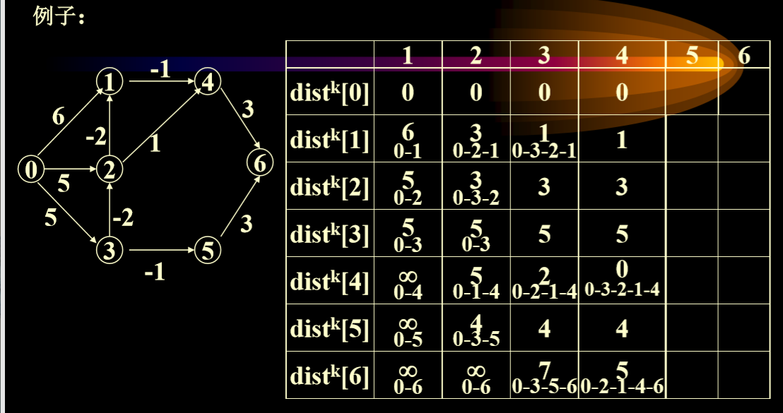
- 更新的时候都是根据前面结果,遍历计算存储
- 所有第k步,只受第k-1步的影响
1 | |
- 时间复杂度:O(n3)
6.3. floyed算法
- 前提:各边权值均大于0的带权有向图。
- 每个顶点到自己的代价为0
- 方法:
- 把有向图的每一个顶点作为源点,重复执行Dijkstra算法n次,执行时间为O(n3)
- Floyed方法,算法形式更简单些,但是时间仍然是O(n3)


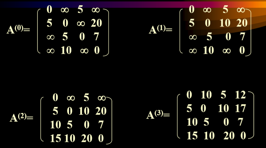
- 简单来说就是:每次都会选择一个中介点,然后遍历整个数组,更新相应的需要更新的数组。
6.3.1. floyed算法实现
1 | |
- 算法复杂度:O(n3)
- 参考:Floyed算法
6.4. Floyed算法参考
7. 活动网络(图的应用)
- 用顶点表示活动的网络(AOV网络)
- 用边表示活动的网络(AOE网络)
- 用顶点表示活动的网络
7.1. AOV网络
7.1.1. AOV网络结构
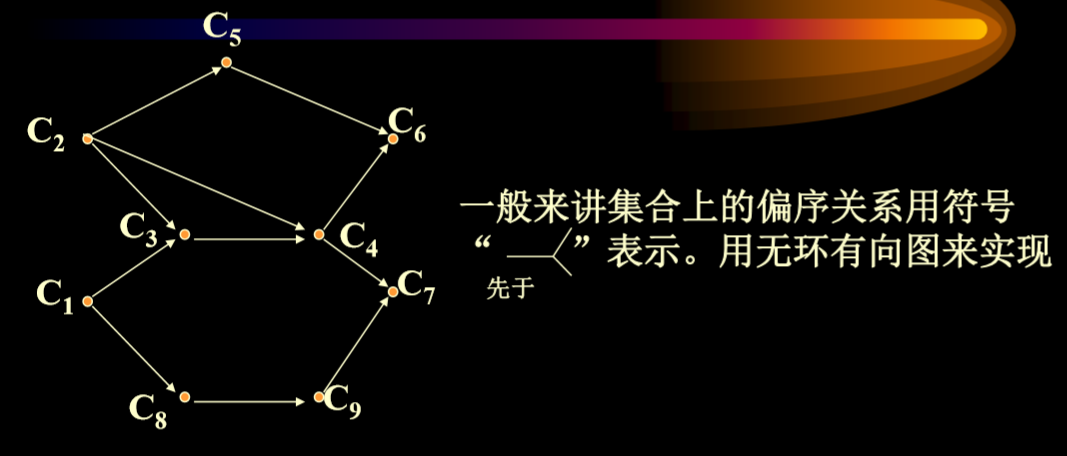
- 图中顶点表示课程(活动),有向边(弧)表示先决条件。 若课程i是课程j的预修课程,则图中有弧<i,j>
- AOV网(Activity On Vertex network)
- 用顶点表示活动,用弧表示活动间的优先关系的有向图称为AOV网。
- 直接前驱,直接后继
- <i,j>是网中一条弧,则i是j的直接前驱,j是i的直接后继。
- 前驱,后继
- 从顶点i->顶点j有一条有向路径,则称i是j的前驱,j是i的后继。
- AOV网中,不应该出现有向环
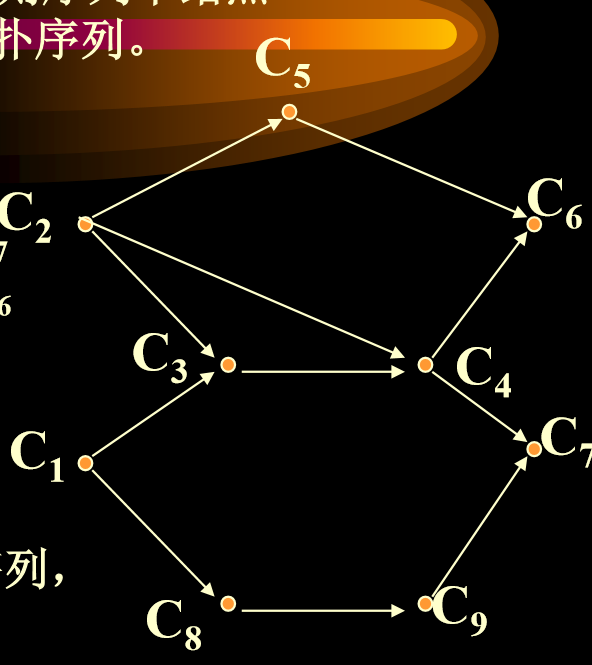
7.1.2. AOV图的拓扑排序
- 有向图G=(V,E),V里结点的线性序列(vi1,vi2,…,vin), 如果满足: 在G中从结点 vi 到 vj 有一条路径,则序列中结点 Vi 必先于结点 vj ,称这样的线性序列为一拓扑序列。
- 不是任何有向图的结点都可以排成拓扑序列,有环图是显然没有拓扑排序的。
7.1.3. 拓扑算法思想
- 从图中选择一个入度为0的结点输出之。(如果一个图中,同时存在多个入度为0的结点,则随便输出任意一个结点)
- 从图中删掉此结点及其所有的出边。
- 反复执行以上步骤
- 直到所有结点都输出了,则算法结束
- 如果图中还有结点,但入度不为0,则说明有环路
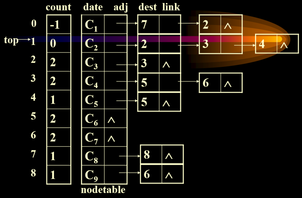
7.1.4. 拓扑算法实现
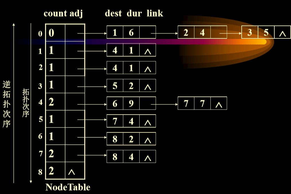
- 具体实现算法:AOV网用邻接表来实现数组count存放各顶点的入度
- 并且为了避免每次从头到尾查找入度为0的顶点,建立入度为0的顶点栈,栈顶指针为top,初始化时为-1.
1 | |
- java实现
1 | |
7.1.5. 算法复杂度分析
- 算法分析:n个顶点,e条边
- 建立链式栈O(n),每个结点输出一次,每条边被检查一次O(n+e),所以为:O(n+n+e)
7.2. AOE网络
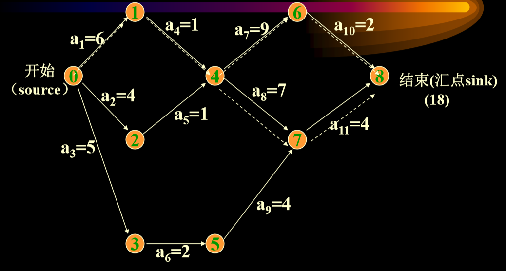
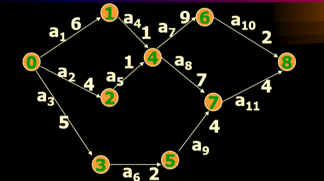
- 用边表示活动的网络(AOE网络, Activity On Edge Network)又称为事件顶点网络
- 顶点:
- 表示事件(event) 事件——状态。表示它的入边代表的活动已完成,它的出边 代表的活动可以开始,如下图v0表示整个工程开始,v4表示a4,a5活动已完成a7,a8活动可开始。
- 有向边:
- 表示活动。 边上的权——表示完成一项活动需要的时间

7.2.1. 关键路径
- 目的: 利用事件顶点网络,研究完成整个工程需要多少时间 加快那些活动的速度后,可使整个工程提前完成。
- 关键路径:具有从开始顶点(源点)->完成顶点(汇点)的 最长的路径
7.2.2. 一些定义
- 对于事件:
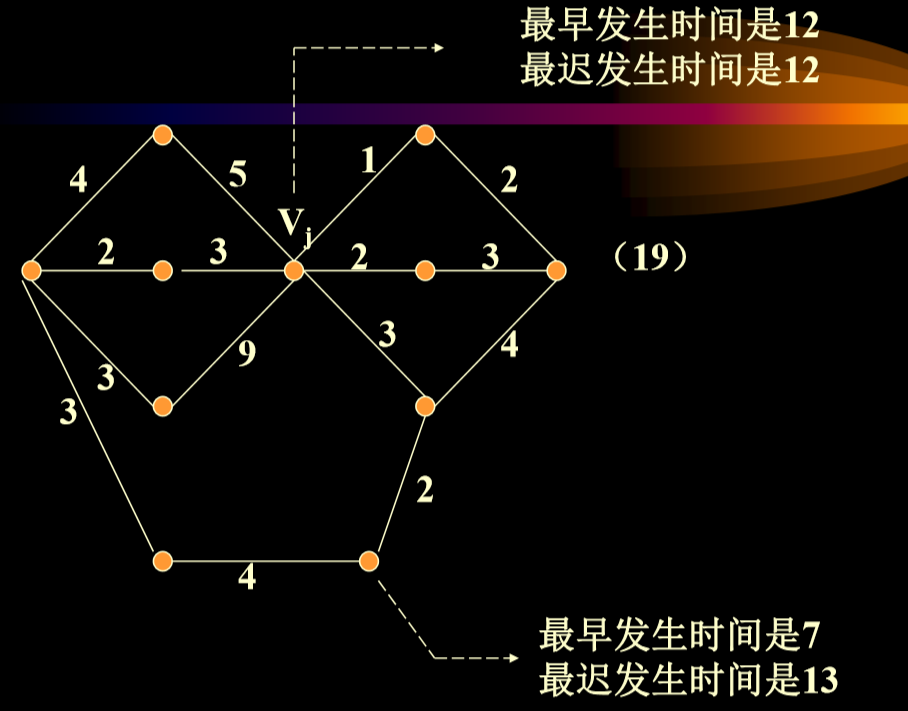
- Ve[i]-表示事件Vi的可能最早发生时间:定义为从源点V0->Vi的最长路径长度, 如Ve[4]=7天
- Vl[i]-表示事件Vi的允许的最晚发生时间:是在保证汇点 Vn-1 在Ve[n-1]时刻(18)完成的前提下,事件Vi允许发生的最晚时间= Ve[n-1]- Vi->Vn-1的最长路径长度。是从最后汇点时间长度-两者之间最长路径
-
解释:
- 计算到最后汇点的总共最短时间:找到从源点到汇点的最大路径
- 最早12,因为之前不能做。
- 最晚12,是因为如果这时候不开始,最后完成不了。
-
对于活动:
- e[k]-表示活动ak=<Vi,Vj>的可能的最早开始时间。 即等于事件Vi的可能最早发生时间。 e[k]=Ve[i]
- l[k]-表示活动ak= <Vi,Vj> 的允许的最迟开始时间 l[k]=Vl[j]-dur(<i,j>);
- l[k]-e[k]-表示活动ak的最早可能开始时间和最迟允许开始时间的时间余量。也称为松弛时间。 (slack time)
- l[k]==e[k]-表示活动ak是没有时间余量的关键活动
-
一开始的例子中
- a8的最早可能开始时间e[8]=Ve[4]=7
- 最迟允许开始时间l[8]=Vl[7]-dur(<4,7>) =14-7=7,所以a8是关键路径上的关键活动
- a9的最早可能开始时间e[9]=Ve[5]=7
- 最迟允许开始时间l[9]=Vl[7]-dur(<5,7>) =14-4=10
-
所以l[9]-e[9]=3, 该活动的时间余量为3,即推迟3天或延迟3天完成都不 影响整个工程的完成,它不是关键活动
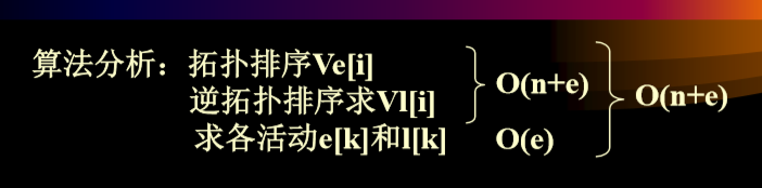
7.2.3. 寻找关键路径的算法
- 求各事件的可能最早发生时间 从Ve[0]=0开始,向前推进求其它事件的Ve Ve[i]=max{Ve[j]+dur(< Vj,Vi >)}, <Vj,Vi>属于S2, i=1,2,…n-1 j S2是所有指向顶点Vi的有向边< Vj,Vi >的集合
- 求各事件的允许最晚发生时间 从Vl[n-1]=Ve[n-1]开始,反向递推 Vl[i]=min{Vl[j]-dur (<Vi,Vj>)}, <Vi,Vj>属于S1, i=n-2,n-3,…0 j S1是所有从顶点Vi出发的有向边< Vi,Vj >的集合
- 以上的计算必须在拓扑有序及逆拓扑有序的前提下进行,求Ve[i]必须使Vi的所有前驱结点的Ve都求得求Vl[i]必须使Vi的所有后继结点最晚发生时间都求得。
- 求每条边(活动)ak= <Vi,Vj> 的e[k], l[k] e[k]=Ve[i];l[k]=Vl[j]-dur(<Vi,Vj> ),k=1,2,…e
- 如果e[k]==l[k],则ak是关键活动
- AOE网用邻接表来表示,并且假设顶点序列已按拓扑有序与逆拓扑有序排好。如上例:
- 先正向推,然后反向推回来。(分别计算最早时间和最晚时间)
7.2.4. 算法实现
1 | |
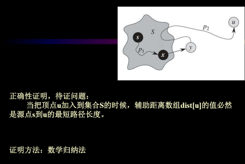
8. 2009年统考题(综合应用题)
带权图 ( 权值非负, 表示边连接的两顶点间的距离) 的最短路径 问题是找出从初始顶点到目标顶点之间的一条最短路径. 假设从初始 顶点到目标顶点之间存在路径, 现有一种解决该问题的方法:
- 设最短路径初始时仅包含初始顶点, 令当前顶点u为初始顶点;
- 选择离u 最近且尚未在最短路径中的一个顶点v, 加入到最短路径中, 修改当前顶点 u = v ;
- 重复步骤2), 直到u是目标顶点时为止. 请问上述方法能否求得最短路径? 若该方法可行, 请证明之; 否则, 请举例说明.
- 不可行,可能取到的是局部最优解
2019-数据结构-数据结构8.0-graphs
https://spricoder.github.io/2020/01/17/2019-Data-Structure/2019-Data-Structure-%E6%95%B0%E6%8D%AE%E7%BB%93%E6%9E%848.0-graphs/